Mixture of Experts (MoE)
A neural network architecture that uses multiple specialized “expert” sub-networks, with a gating mechanism that routes each input to only the most relevant experts, enabling massive model capacity while keeping computational costs low by activating only a fraction of parameters per input.
The Simple Version
Imagine a hospital with many specialists: cardiologists, neurologists, orthopedic surgeons, etc. When a patient arrives, they don’t see all the doctors — a triage nurse (the “gate”) routes them to the right specialist based on their symptoms. Only the relevant experts work on that case.
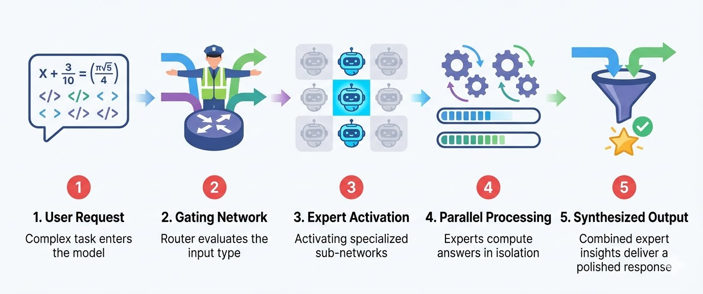
Mixture of Experts works the same way. The model has many “expert” sub-networks, each specializing in different types of inputs. A gating mechanism decides which experts to activate for each input. This means you can have a huge model (many experts) but only use a small part of it for each input, keeping computation fast and cheap.
For example, Mixtral 8x7B has 8 expert networks but only uses 2 per input. It has the knowledge capacity of a 47B parameter model but the speed of a 13B model.
Visual Workflow
Detailed Explanation
MoE architectures address the scaling challenge: how do you make models bigger (more knowledge) without making them proportionally slower and more expensive?
Core Components:
1. Expert Networks:
- Multiple feed-forward networks (or other sub-networks)
- Each expert learns to specialize in different input patterns
- Typically 4-64 experts in modern implementations
2. Gating Network (Router):
- Small neural network that decides which experts to use
- Outputs probabilities for each expert
- Selects top-K experts (usually K=2)
- Can be learned or heuristic-based
3. Sparse Activation:
- Only selected experts process each input
- Other experts remain inactive (computationally free)
- Dramatically reduces FLOPs per token
MoE Variants:
1. Sparse MoE (Standard):
- Top-K experts activated per token
- Most common in LLMs (Mixtral, GPT-4 rumored)
- Example: 8 experts, use top 2
2. Dense MoE:
- All experts process all inputs
- Less common, more like ensemble learning
- Higher compute but better gradient flow
3. Hierarchical MoE:
- Experts organized in hierarchy
- Higher-level gates route to lower-level expert groups
- Enables even larger scale
4. Expert Choice MoE:
- Experts choose which tokens to process (vs. tokens choosing experts)
- Better load balancing
- Used in some recent models
Key Benefits:
- Capacity vs. Compute: Large knowledge capacity, low inference cost
- Specialization: Experts learn domain-specific patterns
- Scalability: Can scale to trillions of parameters efficiently
- Efficiency: 3-5x faster than dense models of same capacity
Challenges:
- Load Balancing: Ensuring all experts are used (some may be ignored)
- Training Instability: Sparse gradients can cause issues
- Communication Overhead: Distributed MoE requires expert parallelism
- Memory: All experts must be loaded even if not all are active
Key Characteristics
- Sparse Activation: Only a fraction of parameters active per input
- Scalable: Enables trillion-parameter models efficiently
- Specialized: Experts learn different patterns
- Efficient: High capacity, low compute cost
- Complex: Harder to train and deploy than dense models
Business Context
MoE is becoming the standard architecture for frontier LLMs:
Why MoE Matters:
- Cost Efficiency: Serve large models at lower cost per token
- Performance: Achieve better quality than dense models at same compute
- Scalability: Scale to larger models without proportional cost increase
- Competitive Advantage: Leading models (GPT-4, Mixtral, Claude) use MoE
Enterprise Implications:
- Model Selection: MoE models offer better price-performance ratio
- Deployment: MoE models require specialized serving infrastructure
- Fine-tuning: PEFT methods (LoRA) work well with MoE
- Vendor Evaluation: Understand if vendor models are MoE (affects pricing)
Popular MoE Models:
- Mixtral 8x7B: Open-source, 8 experts, top-2 routing
- GPT-4: Rumored to be MoE (not confirmed by OpenAI)
- Claude 3: Likely uses MoE architecture
- DBRX: Databricks’ open-source MoE model
- Qwen-MoE: Alibaba’s MoE implementation
Cost Comparison:
- Dense 70B model: ~$0.06 per 1M tokens
- MoE 8x7B model: ~$0.02 per 1M tokens (similar quality, 3x cheaper)
Real-World Analogy
A consulting firm with many specialists. For each client project, the firm doesn’t assign all consultants — just the 2-3 most relevant experts. The firm has deep expertise across many domains (high capacity) but only pays the relevant experts for each project (low cost). This is MoE in action.
Code Example
# Conceptual MoE layer in PyTorch
import torch
import torch.nn as nn
import torch.nn.functional as F

class MoELayer(nn.Module):
    def __init__(self, dim, num_experts=8, top_k=2):
        super().__init__()
        self.num_experts = num_experts
        self.top_k = top_k

        # Create expert networks
        self.experts = nn.ModuleList([
            nn.Sequential(
                nn.Linear(dim, dim * 4),
                nn.GELU(),
                nn.Linear(dim * 4, dim)
            )
            for _ in range(num_experts)
        ])

        # Gating network
        self.gate = nn.Linear(dim, num_experts)

    def forward(self, x):
        # x shape: [batch, seq_len, dim]
        batch_size, seq_len, dim = x.shape

        # Compute gating scores
        gate_scores = self.gate(x)  # [batch, seq_len, num_experts]
        gate_probs = F.softmax(gate_scores, dim=-1)

        # Select top-K experts
        top_k_probs, top_k_indices = torch.topk(gate_probs, self.top_k, dim=-1)

        # Normalize probabilities
        top_k_probs = top_k_probs / top_k_probs.sum(dim=-1, keepdim=True)

        # Process through selected experts
        output = torch.zeros_like(x)

        for i in range(self.top_k):
            expert_idx = top_k_indices[:, :, i]
            expert_prob = top_k_probs[:, :, i:i+1]

            # Route to appropriate expert
            for b in range(batch_size):
                for s in range(seq_len):
                    expert = self.experts[expert_idx[b, s]]
                    expert_output = expert(x[b:b+1, s:s+1])
                    output[b:b+1, s:s+1] += expert_prob[b, s] * expert_output

        return output

# Usage
moe_layer = MoELayer(dim=512, num_experts=8, top_k=2)
x = torch.randn(2, 10, 512)  # [batch=2, seq=10, dim=512]
output = moe_layer(x)
print(f"Input shape: {x.shape}, Output shape: {output.shape}")
Common Misconceptions
- Myth: MoE models are just ensembles of separate models.
-
Reality: MoE models share lower layers (embeddings, attention) and only have experts in specific layers (usually feed-forward). They’re integrated architectures, not separate models.
- Myth: MoE is always better than dense models.
-
Reality: MoE excels at scale but adds complexity. For smaller models (<10B), dense architectures are often simpler and perform equally well.
- Myth: MoE models use all their parameters for each input.
-
Reality: Only a fraction of parameters are active per input (e.g., 2 out of 8 experts). This is what makes MoE efficient.
- Myth: MoE models are harder to fine-tune.
- Reality: PEFT methods like LoRA work well with MoE. You can fine-tune specific experts or add LoRA adapters to experts.